大家好，我是小寒。

今天给大家分享一个超强的算法模型，Vision Transformer

Vision Transformer（ViT）是一种基于自注意力机制的神经网络架构，主要用于处理图像数据。

它是由谷歌研究人员在 2020 年提出的，标志着将自然语言处理（NLP）中广泛使用的 Transformer 模型成功应用于计算机视觉领域的一个重要进展。

基本原理和架构

Vision Transformer 的核心思想是将图像分解为一系列的小块（称为 patches），这些小块在输入网络之前被展平并映射到高维空间。这与传统的卷积神经网络（CNN）不同，后者通常会使用卷积层来处理整个图像并提取局部特征。

1.图像分块

首先，ViT 将输入图像切割成固定大小的小块（例如，16x16像素的块）。每个块被视为一个 “token”，与 NLP 中的单词类似。

2.嵌入层

这些图像块（patches）被展平并通过一个线性层转换成一系列的嵌入向量。

此外，还会添加一个可学习的 “类别” 嵌入，用于聚合全局信息。

3.位置编码

为了保留图像块的位置信息，ViT 在嵌入向量中加入位置编码，这是 Transformer 架构中的一个关键组成部分。

4.Transformer 编码器

经过嵌入的图像块（现在作为序列的一部分）输入到标准的 Transformer编码器中。

编码器使用多头自注意力机制和前馈神经网络来处理序列，允许模型捕获块之间的复杂关系。

关于 Transformer 编码器的细节，可以参考下面这篇文章。

5.分类头

对于分类任务，Transformer 的输出（特别是 [CLS] token 的输出）会传递到一个前馈网络（即分类头），该网络输出最终的类别预测。

优缺点分析

Vision Transformer (ViT) 和卷积神经网络（CNN）都是处理图像任务的流行模型，下面我们来比较一下它们的优缺点。

VIT

优点

• 强大的全局信息处理能力

通过自注意力机制，ViT 可以在图像的任何部分之间建立直接的联系，有效捕捉全局依赖关系。

• 高度灵活性

ViT 模型可以很容易地调整到不同大小的输入，且模型架构可扩展性强。

• 更适合大规模数据集

ViT 在大规模数据集上表现通常优于传统 CNN，可以学习更复杂的视觉模式。

缺点

• 需要更多的训练数据

ViT 依赖大量数据来训练，以防止过拟合，对于数据较少的情况可能不如CNN有效。

• 计算成本高

由于需要计算长距离的依赖关系，ViT 在计算和内存需求上通常比CNN要高。

CNN

优点

• 局部感知能力强

非常适合捕捉局部的视觉模式，如边缘，这在图像处理中非常重要。

• 参数更少

由于共享权重和局部连接，CNN 通常比 ViT 更节省参数，易于训练和泛化。

• 计算效率

在小规模数据集上，CNN 通常更高效，并且需要的计算资源较少。

缺点

• 有限的感受野

需要通过堆叠多层卷积层才能扩展感受野，对全局信息的捕获不如 ViT。

• 固定的结构

卷积核的大小和步长是固定的，可能限制了模型处理不同尺度特征的能力。

代码实现

1.图像分块

import os
import copy
import math
import typing
import cv2
import numpy as np
import matplotlib.pyplot as plt
import torch
import torch.nn as nn
mountains = np.load('mountains.npy')
H = mountains.shape[0]
W = mountains.shape[1]
print('Mountain at Dusk is H =', H, 'and W =', W, 'pixels.')
P = 20
N = int((H*W)/(P**2))
print('There will be', N, 'patches, each', P, 'by', str(P)+'.')
fig = plt.figure(figsize=(10,6))
plt.imshow(mountains, cmap='Purples_r')
plt.hlines(np.arange(P, H, P)-0.5, -0.5, W-0.5, color='w')
plt.vlines(np.arange(P, W, P)-0.5, -0.5, H-0.5, color='w')
plt.xticks(np.arange(-0.5, W+1, 10), labels=np.arange(0, W+1, 10))
plt.yticks(np.arange(-0.5, H+1, 10), labels=np.arange(0, H+1, 10))
x_text = np.tile(np.arange(9.5, W, P), 3)
y_text = np.repeat(np.arange(9.5, H, P), 5)
for i in range(1, N+1):
    plt.text(x_text[i-1], y_text[i-1], str(i), color='w', fontsize='xx-large', ha='center')
plt.text(x_text[2], y_text[2], str(3), color='k', fontsize='xx-large', ha='center');

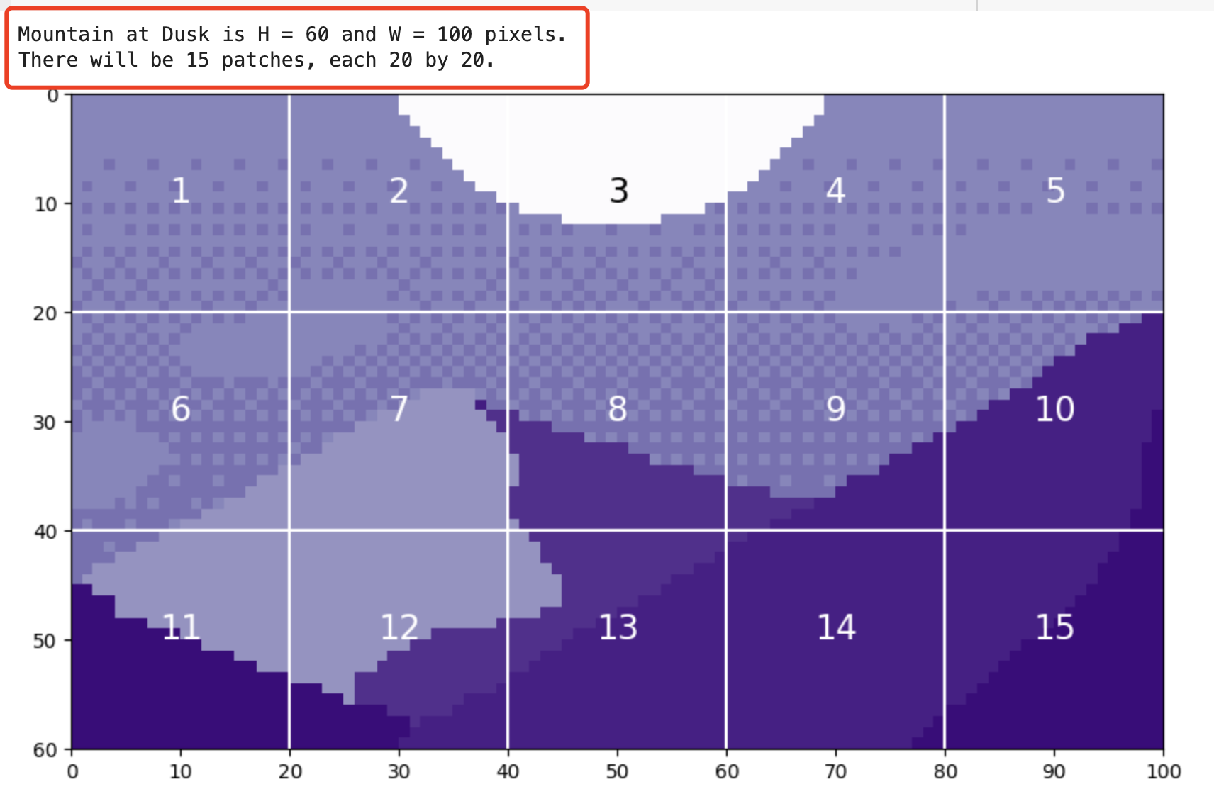
通过展平这些色块，我们可以看到生成的 token。我们以色块 12 为例，因为它包含四种不同的色调。

print('Each patch will make a token of length', str(P**2)+'.')

patch12 = mountains[40:60, 20:40]
token12 = patch12.reshape(1, P**2)
fig = plt.figure(figsize=(10,1))
plt.imshow(token12, aspect=10, cmap='Purples_r')
plt.clim([0,1])
plt.xticks(np.arange(-0.5, 401, 50), labels=np.arange(0, 401, 50))
plt.yticks([])

2.嵌入层

从图像中提取 token 后，通常使用线性投影来更改 token 的长度。

现在我们理解了这个概念，我们可以看看补丁标记化是如何在代码中实现的。

class Patch_Tokenization(nn.Module):
    def __init__(self,
                img_size: tuple[int, int, int]=(1, 1, 60, 100),
                patch_size: int=50,
                token_len: int=768):

        super().__init__()
        self.img_size = img_size
        C, H, W = self.img_size
        self.patch_size = patch_size
        self.token_len = token_len
        assert H % self.patch_size == 0, 'Height of image must be evenly divisible by patch size.'
        assert W % self.patch_size == 0, 'Width of image must be evenly divisible by patch size.'
        self.num_tokens = (H / self.patch_size) * (W / self.patch_size)

        ## Defining Layers
        self.split = nn.Unfold(kernel_size=self.patch_size, stride=self.patch_size, padding=0)
        self.project = nn.Linear((self.patch_size**2)*C, token_len)

    def forward(self, x):
        x = self.split(x).transpose(1,0)
        x = self.project(x)
        return x

请注意，这两个 assert 语句确保图像尺寸可以被块大小整除。实际分割成块的操作是使用 torch.nn.Unfold 层实现的。

x = torch.from_numpy(mountains).unsqueeze(0).unsqueeze(0).to(torch.float32)
token_len = 768
print('Input dimensions are\n\tbatchsize:', x.shape[0], '\n\tnumber of input channels:', x.shape[1], '\n\timage size:', (x.shape[2], x.shape[3]))

# Define the Module
patch_tokens = Patch_Tokenization(img_size=(x.shape[1], x.shape[2], x.shape[3]),
                                    patch_size = P,
                                    token_len = token_len)

x = patch_tokens.split(x).transpose(2,1)
print('After patch tokenization, dimensions are\n\tbatchsize:', x.shape[0], '\n\tnumber of tokens:', x.shape[1], '\n\ttoken length:', x.shape[2])

x = patch_tokens.project(x)
print('After projection, dimensions are\n\tbatchsize:', x.shape[0], '\n\tnumber of tokens:', x.shape[1], '\n\ttoken length:', x.shape[2])

从上图可以看到，经过 线性投影层后，token 的维度变成了 768。

3.位置编码

接下来将一个空白 token（称为预测标记）添加到图像 token 之前。此 token 将在编码块的输出中用于进行预测。

它从空白（相当于零）开始，以便它可以从其他图像标记中获取信息。

pred_token = torch.zeros(1, 1, x.shape[2]).expand(x.shape[0], -1, -1)
x = torch.cat((pred_token, x), dim=1)

然后，我们为 token 添加一个位置嵌入。

位置嵌入允许 transformer 理解图像标记的顺序。

def get_sinusoid_encoding(num_tokens, token_len):

    def get_position_angle_vec(i):
        return [i / np.power(10000, 2 * (j // 2) / token_len) for j in range(token_len)]

    sinusoid_table = np.array([get_position_angle_vec(i) for i in range(num_tokens)])
    sinusoid_table[:, 0::2] = np.sin(sinusoid_table[:, 0::2])
    sinusoid_table[:, 1::2] = np.cos(sinusoid_table[:, 1::2]) 

    return torch.FloatTensor(sinusoid_table).unsqueeze(0)



PE = get_sinusoid_encoding(x.shape[1]+1, x.shape[2])
print('Position embedding dimensions are\n\tnumber of tokens:', PE.shape[1], '\n\ttoken length:', PE.shape[2])

x = x + PE
print('Dimensions with Position Embedding are\n\tbatchsize:', x.shape[0], '\n\tnumber of tokens:', x.shape[1], '\n\ttoken length:', x.shape[2])

4.编码器

编码器是模型实际从图像 token 中学习的地方。

编码器主要由注意力模块和神经网络模块组成。

NoneFloat = typing.Union[None, float]
class Attention(nn.Module):
    def __init__(self, 
                dim: int,
                chan: int,
                num_heads: int=1,
                qkv_bias: bool=False, qk_scale: NoneFloat=None):

        super().__init__()


        self.num_heads = num_heads
        self.chan = chan
        self.head_dim = self.chan // self.num_heads
        self.scale = qk_scale or self.head_dim ** -0.5

        self.qkv = nn.Linear(dim, chan * 3, bias=qkv_bias)
        self.proj = nn.Linear(chan, chan)

    def forward(self, x):
        if self.chan % self.num_heads != 0:
            raise ValueError('"Chan" must be evenly divisible by "num_heads".')
        B, N, C = x.shape
        qkv = self.qkv(x).reshape(B, N, 3, self.num_heads, self.head_dim).permute(2, 0, 3, 1, 4)

        q, k, v = qkv[0], qkv[1], qkv[2]

        ## Calculate Attention
        attn = (q * self.scale) @ k.transpose(-2, -1)
        attn = attn.softmax(dim=-1)

        x = (attn @ v).transpose(1, 2).reshape(B, N, self.chan)
        x = self.proj(x)

        ## Skip Connection Layer
        v = v.transpose(1, 2).reshape(B, N, self.chan)
        x = v + x     
        return x

class NeuralNet(nn.Module):
    def __init__(self,
       in_chan: int,
       hidden_chan: NoneFloat=None,
       out_chan: NoneFloat=None,
       act_layer = nn.GELU):

        super().__init__()

        ## Define Number of Channels
        hidden_chan = hidden_chan or in_chan
        out_chan = out_chan or in_chan

        ## Define Layers
        self.fc1 = nn.Linear(in_chan, hidden_chan)
        self.act = act_layer()
        self.fc2 = nn.Linear(hidden_chan, out_chan)

    def forward(self, x):
        x = self.fc1(x)
        x = self.act(x)
        x = self.fc2(x)
        return x

class Encoding(nn.Module):
    def __init__(self,
       dim: int,
       num_heads: int=1,
       hidden_chan_mul: float=4.,
       qkv_bias: bool=False,
       qk_scale: NoneFloat=None,
       act_layer=nn.GELU, 
       norm_layer=nn.LayerNorm):

        super().__init__()

        ## Define Layers
        self.norm1 = norm_layer(dim)
        self.attn = Attention(dim=dim,
                            chan=dim,
                            num_heads=num_heads,
                            qkv_bias=qkv_bias,
                            qk_scale=qk_scale)
        self.norm2 = norm_layer(dim)
        self.neuralnet = NeuralNet(in_chan=dim,
                                hidden_chan=int(dim*hidden_chan_mul),
                                out_chan=dim,
                                act_layer=act_layer)

    def forward(self, x):
        x = x + self.attn(self.norm1(x))
        x = x + self.neuralnet(self.norm2(x))
        return x

现在，我们将通过一个规范层和一个注意力模块。

E = Encoding(dim=x.shape[2], num_heads=4, hidden_chan_mul= 1.5 , qkv_bias= False , qk_scale= None , act_layer=nn.GELU, norm_layer=nn.LayerNorm) 
y = E.norm1(x)
print('After norm, dimensions are\n\tbatchsize:', y.shape[0], '\n\tnumber of tokens:', y.shape[1], '\n\ttoken size:', y.shape[2])
y = E.attn(y)
print('After attention, dimensions are\n\tbatchsize:', y.shape[0], '\n\tnumber of tokens:', y.shape[1], '\n\ttoken size:', y.shape[2])
y = y + x
print('After split connection, dimensions are\n\tbatchsize:', y.shape[0], '\n\tnumber of tokens:', y.shape[1], '\n\ttoken size:', y.shape[2])

接下来，我们经过神经网络模块。

z = E.norm2(y)
print('After norm, dimensions are\n\tbatchsize:', z.shape[0], '\n\tnumber of tokens:', z.shape[1], '\n\ttoken size:', z.shape[2])
z = E.neuralnet(z)
print('After neural net, dimensions are\n\tbatchsize:', z.shape[0], '\n\tnumber of tokens:', z.shape[1], '\n\ttoken size:', z.shape[2])
z = z + y
print('After split connection, dimensions are\n\tbatchsize:', z.shape[0], '\n\tnumber of tokens:', z.shape[1], '\n\ttoken size:', z.shape[2])

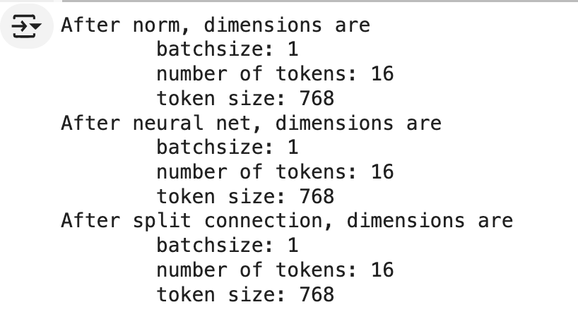
这就是单个编码器的全部内容！由于最终尺寸与初始尺寸相同，因此模型可以轻松地将 token 传递到多个编码器。

5.分类头

经过编码器后，模型要做的最后一件事就是进行预测。

norm = nn.LayerNorm(token_len)
z = norm(z)
pred_token = z[:, 0]
head = nn.Linear(pred_token.shape[-1], 1)
pred = head(pred_token)
print('Length of prediction:', (pred.shape[0], pred.shape[1]))
print('Prediction:', float(pred))

整体代码

class ViT_Backbone(nn.Module):
    def __init__(self,
                preds: int=1,
                token_len: int=768,
                num_heads: int=1,
                Encoding_hidden_chan_mul: float=4.,
                depth: int=12,
                qkv_bias=False,
                qk_scale=None,
                act_layer=nn.GELU,
                norm_layer=nn.LayerNorm):

        super().__init__()

        ## Defining Parameters
        self.num_heads = num_heads
        self.Encoding_hidden_chan_mul = Encoding_hidden_chan_mul
        self.depth = depth

        ## Defining Token Processing Components
        self.cls_token = nn.Parameter(torch.zeros(1, 1, self.token_len))
        self.pos_embed = nn.Parameter(data=get_sinusoid_encoding(num_tokens=self.num_tokens+1, token_len=self.token_len), requires_grad=False)

        ## Defining Encoding blocks
        self.blocks = nn.ModuleList([Encoding(dim = self.token_len, 
                                               num_heads = self.num_heads,
                                               hidden_chan_mul = self.Encoding_hidden_chan_mul,
                                               qkv_bias = qkv_bias,
                                               qk_scale = qk_scale,
                                               act_layer = act_layer,
                                               norm_layer = norm_layer)
             for i in range(self.depth)])

        ## Defining Prediction Processing
        self.norm = norm_layer(self.token_len)
        self.head = nn.Linear(self.token_len, preds)

        ## Make the class token sampled from a truncated normal distrobution 
        timm.layers.trunc_normal_(self.cls_token, std=.02)

    def forward(self, x):
        ## Assumes x is already tokenized

        ## Get Batch Size
        B = x.shape[0]
        ## Concatenate Class Token
        x = torch.cat((self.cls_token.expand(B, -1, -1), x), dim=1)
        ## Add Positional Embedding
        x = x + self.pos_embed
        ## Run Through Encoding Blocks
        for blk in self.blocks:
            x = blk(x)
        ## Take Norm
        x = self.norm(x)
        ## Make Prediction on Class Token
        x = self.head(x[:, 0])
        return x



class ViT_Model(nn.Module):
 def __init__(self,
    img_size: tuple[int, int, int]=(1, 400, 100),
    patch_size: int=50,
    token_len: int=768,
    preds: int=1,
    num_heads: int=1,
    Encoding_hidden_chan_mul: float=4.,
    depth: int=12,
    qkv_bias=False,
    qk_scale=None,
    act_layer=nn.GELU,
    norm_layer=nn.LayerNorm):

  super().__init__()

  ## Defining Parameters
  self.img_size = img_size
  C, H, W = self.img_size
  self.patch_size = patch_size
  self.token_len = token_len
  self.num_heads = num_heads
  self.Encoding_hidden_chan_mul = Encoding_hidden_chan_mul
  self.depth = depth

  ## Defining Patch Embedding Module
  self.patch_tokens = Patch_Tokenization(img_size,
           patch_size,
           token_len)

  ## Defining ViT Backbone
  self.backbone = ViT_Backbone(preds,
         self.token_len,
         self.num_heads,
         self.Encoding_hidden_chan_mul,
         self.depth,
         qkv_bias,
         qk_scale,
         act_layer,
         norm_layer)
  ## Initialize the Weights
  self.apply(self._init_weights)

 def _init_weights(self, m):
  """ Initialize the weights of the linear layers & the layernorms
  """
  ## For Linear Layers
  if isinstance(m, nn.Linear):
   ## Weights are initialized from a truncated normal distrobution
   timm.layers.trunc_normal_(m.weight, std=.02)
   if isinstance(m, nn.Linear) and m.bias is not None:
    ## If bias is present, bias is initialized at zero
    nn.init.constant_(m.bias, 0)
  ## For Layernorm Layers
  elif isinstance(m, nn.LayerNorm):
   ## Weights are initialized at one
   nn.init.constant_(m.weight, 1.0)
   ## Bias is initialized at zero
   nn.init.constant_(m.bias, 0)

 @torch.jit.ignore ##Tell pytorch to not compile as TorchScript
 def no_weight_decay(self):
  """ Used in Optimizer to ignore weight decay in the class token
  """
  return {'cls_token'}

 def forward(self, x):
  x = self.patch_tokens(x)
  x = self.backbone(x)
  return x